Hybrid Logical Clocks: Causality and Wall Time Without Coordination

Distributed systems have a time problem that isn't obvious until it bites you.
Two events happened — one on Node A, one on Node B. Which came first? That question has two different answers depending on what you mean by "first": physical time order, or causal order. The answer you need depends on what you're building. And the disturbing reality is that neither physical clocks nor Lamport clocks can give you both, simultaneously, cheaply. HLC does. It fits in 64 bits, runs on commodity hardware, and requires no global coordinator.
Why physical clocks fail at causality
Physical clocks drift. Even with NTP, real-world deployments see skew of 200–500ms between nodes on commodity infrastructure. Google's Spanner paper reported skew of several milliseconds even with GPS and atomic clocks.
Here's what that skew means concretely. Node A writes record R at physical time t=100ms and sends a "write complete" to Node B. Node B's clock reads t=90ms when it receives the message — it's 15ms behind. If B timestamps a dependent write using its local clock, that write gets timestamp 91ms. Any system ordering events by physical timestamp now believes the dependent write preceded the record it depends on. Causality is broken, silently, by clock drift.
Why Lamport clocks fail at wall time
Lamport clocks capture causality correctly. The rule is simple: increment on every local event; on receive, take max(local, received) + 1. If e causally precedes f, then L(e) < L(f). Guaranteed.
But the converse doesn't hold. L(e) < L(f) doesn't mean e happened before f in physical time. Lamport values are dimensionless counters — a value of 50,000 might represent events seconds or days apart. You cannot answer "give me all events before 3pm" or "is this read stale by more than five minutes?" with a Lamport clock. Any database that needs consistent snapshots tied to wall time — and every production database does, for backup, CDC, and cross-region reads — needs more than Lamport gives you.
The design space
Four properties you want from a distributed timestamp:
| Property | Physical clocks | Lamport | Vector clocks | HLC |
|---|---|---|---|---|
| Causality: e → f implies ts(e) < ts(f) | ✗ | ✓ | ✓ | ✓ |
| Wall-clock proximity | ✓ | ✗ | ✗ | ✓ |
| Scalar comparison | ✓ | ✓ | ✗ | ✓ |
| Bounded space O(1) | ✓ | ✓ | ✗ (O(n)) | ✓ |
HLC gives you all four on commodity hardware.
The HLC structure
An HLC timestamp is a pair (l, c):
lis the physical component — the maximum physical time this node has ever seen, from its own clock or from messages received. It is a high-water mark, never allowed to decrease.cis a counter that breaks ties when two causally-related events share the samelvalue.
The key insight: l is not the node's own physical clock. It is the furthest-forward physical time the node has observed, either locally or through messages. It propagates through the system like a maximum, ensuring that causally-downstream events never carry a timestamp that looks earlier than the events they depend on.
The algorithm
On a send or local event at node j, where pt_j is the current physical clock reading:
l_prev = l_j
l_j    = max(l_j, pt_j)

if l_j == l_prev:
    c_j = c_j + 1    // physical time hasn't moved — increment counter
else:
    c_j = 0          // physical time advanced — reset counter

emit (l_j, c_j)
On receive of a message with timestamp (l_m, c_m) at node j:
l_prev = l_j
l_j    = max(l_j, l_m, pt_j)

if l_j == l_prev and l_j == l_m:
    c_j = max(c_j, c_m) + 1    // both local and message match — merge and increment
elif l_j == l_prev:
    c_j = c_j + 1              // local was already highest
elif l_j == l_m:
    c_j = c_m + 1              // message carried the highest l — inherit counter
else:
    c_j = 0                    // physical time jumped past both
Ordering: (l₁, c₁) < (l₂, c₂) if and only if l₁ < l₂, or l₁ = l₂ and c₁ < c₂.
This fits in a single 64-bit integer. The Kulkarni-Demirbas paper (2014) suggests 48 bits for l — physical time in milliseconds, enough for centuries — and 16 bits for c, supporting up to 65,535 concurrent events within a single millisecond. CockroachDB uses exactly this layout.
Algorithm trace: two nodes
The following sequence trace shows how HLC timestamps are assigned across two nodes exchanging messages. Pay attention to e2: Node B's physical clock reads 9ms — behind the message's l value of 10. The algorithm takes max(0, 10, 9) = 10, which matches l_m, so the counter increments to preserve the causal ordering: hlc(e2) = (10, 1).
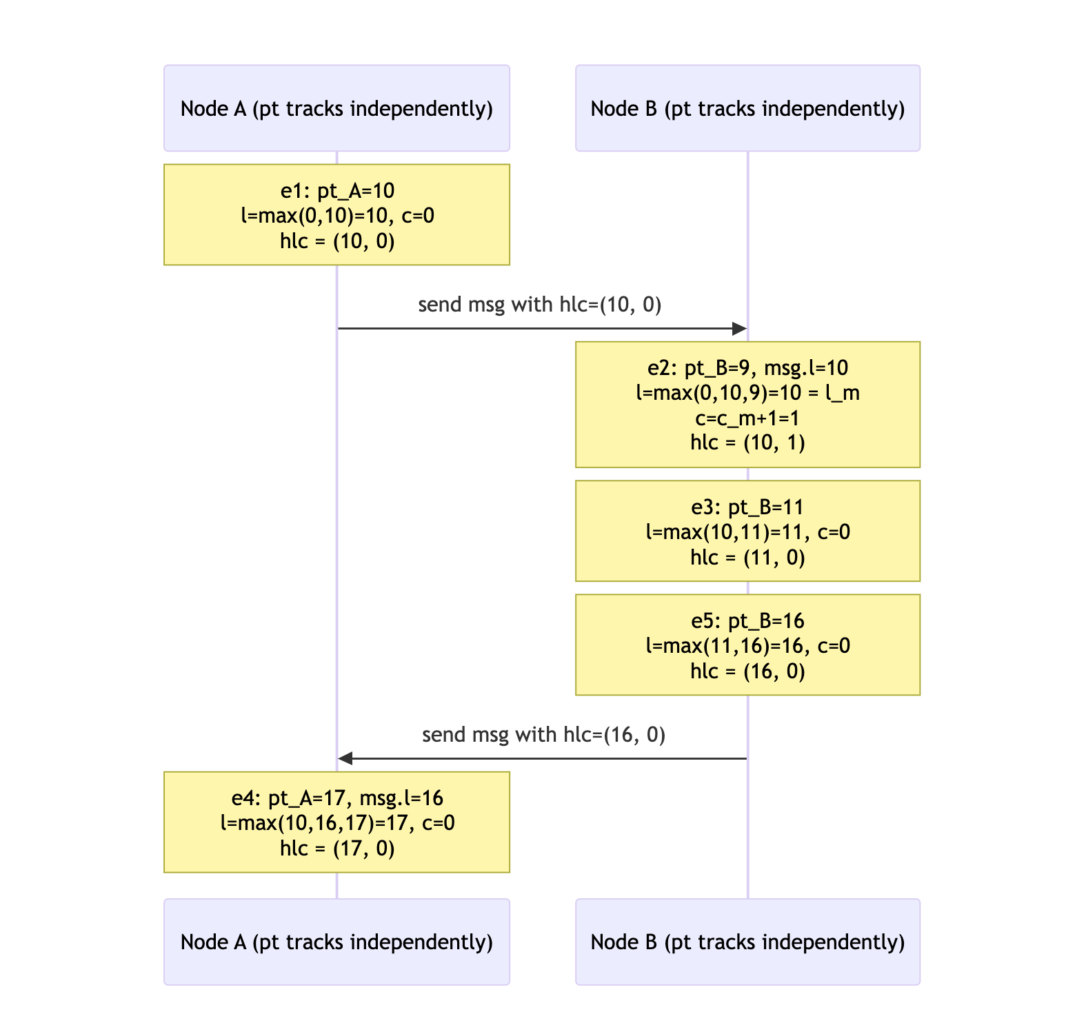
The full causal chain e1 → e2 → e3 → e5 → e4 maps to a strict total order:
(10,0) < (10,1) < (11,0) < (16,0) < (17,0)
Causality is preserved even though B's physical clock was behind A's at the moment of receive.
What the algorithm guarantees
Causality: If e → f (e causally precedes f via the happens-before relation), then hlc(e) < hlc(f). This is the full Lamport property, preserved exactly.
Physical closeness: hlc(e).l ≥ pt(e) always — HLC never goes backward from physical time. The gap is bounded: hlc(e).l − pt(e) ≤ ε, where ε is the maximum clock skew across all nodes. If NTP bounds your skew to 250ms, the l component of any HLC timestamp is never more than 250ms ahead of actual physical time.
Bounded counter: c is bounded by the number of causally-related events sharing the same l value. In any system where the physical clock advances at least once per event, c stays near zero.
Together: you can compare two HLC timestamps with a single 64-bit integer comparison, and when hlc(e).l ≈ hlc(f).l (within clock skew), the comparison reflects actual physical time ordering.
Consistent snapshots without coordination
You want to answer: "give me a consistent view of all data as of time T." Consistent means: if write A causally precedes write B, and B is included in the snapshot, then A must be included too. Miss that property and you get a snapshot of data that could never have existed — referencing a foreign key that wasn't committed yet, reflecting a balance transfer without its corresponding debit.
With HLC, each node answers independently: "return my latest committed state where hlc(commit) ≤ T." Because the l component of HLC captures causality, if B's commit (which depends on A's write) is included in the snapshot, A's write necessarily has a lower HLC — it is included by construction. No coordinator, no synchronization barrier.
The following diagram shows three nodes independently selecting their latest committed event at or before snapshot time T = (15, 0). Each node answers the query locally:
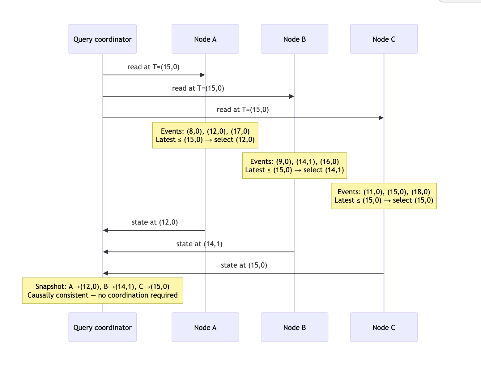
Each node answers independently at query time. The result is causally consistent: any write that influenced a selected event is itself selected, by the monotonicity property of HLC.
Where this runs in production
CockroachDB uses HLC as its primary MVCC timestamp, with exactly the 48-bit/16-bit layout from the original paper. Every committed write gets an HLC timestamp. Reads at a given HLC value return a causally consistent snapshot across all nodes. The closed-timestamp subsystem — which allows followers to serve stale reads without contacting the leaseholder — is built directly on HLC's bounded-skew property.
YugabyteDB calls it "Hybrid Time" and uses the same approach for both its DocDB storage layer and its PostgreSQL-compatible SQL layer. Cross-tablet reads are made consistent by the same mechanism — each tablet independently applies the HLC filter.
MongoDB uses a cluster time with HLC semantics for causally consistent sessions in multi-document transactions. The operationTime field in read responses is an HLC value that can be passed as readConcern.afterClusterTime in subsequent operations — guaranteeing that the later read sees everything the earlier read saw and more.
Apache Cassandra is the instructive counterexample. Cassandra uses client-side physical timestamps with last-write-wins. The documentation explicitly warns about clock skew causing incorrect merge outcomes. This is exactly the gap HLC fills — and the reason every new distributed database built after 2014 uses some variant of it.
TiKV (the storage engine under TiDB) takes a different path: a timestamp oracle (PD, the Placement Driver) issues globally monotonic timestamps on request. This gives tighter bounds and simpler reasoning than HLC, at the cost of a coordination round-trip per transaction start.
HLC versus TrueTime
Google's TrueTime (Spanner, 2012) solves the same problem differently. TrueTime exposes a hardware-backed time API that returns an interval [earliest, latest] instead of a point. Spanner waits out this uncertainty interval before committing (the "commit-wait" step), ensuring that any transaction's commit timestamp is demonstrably in the past before its effects become visible.
TrueTime's uncertainty window averages ~7ms in Google's datacenters. The commit-wait adds this latency to every write transaction. In exchange, you get globally-consistent external consistency with no per-node skew uncertainty.
HLC's guarantee is weaker but cheaper: timestamps are bounded to wall time within the maximum NTP skew ε, and correctness depends on ε being bounded. In practice, with NTP this is 200–500ms; with PTP (Precision Time Protocol) or cloud-provider time sync, it drops to single-digit milliseconds. You don't pay commit-wait, but you need to trust that your clock synchronization infrastructure holds the bound.
| TrueTime | HLC | |
|---|---|---|
| Infrastructure | GPS + atomic clocks | NTP / PTP |
| Write latency overhead | ~7ms commit-wait | ~0ms |
| Clock skew bound | <1ms (hardware) | 200–500ms (NTP), <5ms (PTP) |
| Coordination required | None | None |
| Causality guaranteed | Yes (external consistency) | Yes (happens-before) |
| Snapshot reads | Globally consistent | Causally consistent |
Most consistency bugs in distributed databases aren't in the consensus protocol. The Raft implementation is usually correct. The replication is fine. The bugs are in timestamp semantics — a system that says "we use physical timestamps for ordering" has made a subtle architectural choice to accept causal inconsistency when clocks drift. The inconsistency doesn't show up in unit tests, doesn't show up in integration tests, and surfaces as a corruption report from a production workload under high load when two nodes get slightly out of sync.
HLC is a 64-bit proof of causal position, bounded to wall time within the precision of your clock synchronization infrastructure. It adds two integer comparisons and a counter update to every event — essentially free. The original paper's algorithm fits in eight lines of pseudocode. CockroachDB's implementation fits in a single file.
The timestamp model is an architectural decision, not an implementation detail. Make it deliberately, early, and make it explicit in your code. The 16 lines you write today define what "consistent" means everywhere in your system, forever.